At its core, all modern artificial intelligence is just trying to imitate what you do without thinking.
When you decide whether to cross the street, or whether that email belongs in the spam folder, your brain is processing signals, weighing evidence, and making a simple decision: yes or no.
In artificial neural networks, everything started as an attempt to replicate that behavior in a mathematical model, giving birth to what we know as the Perceptron — still, to this day, one of the most elegant ideas in computing.
Origin
The history of machine learning doesn’t begin with supercomputers, but with pen and paper, back in the 1940s. Here’s a brief timeline:
- 1943 - Artificial Neuron (McCulloch & Pitts): the starting point was a mathematical model of the biological neuron. It was a purely logical structure: if the inputs summed to a value X, the neuron fired. The problem? It didn’t learn — all the rules had to be defined manually.
- 1958 - Perceptron (Frank Rosenblatt): this introduced the concept of weights. For the first time, the algorithm could adjust the importance it assigned to each input based on its mistakes. If it got the answer wrong, it tweaked the weights until it got it right. It was one of the first models with a real capacity to learn.
- 1969 - The AI Winter (Marvin Minsky & Seymour Papert): a book was published proving that the original Perceptron couldn’t solve simple problems like XOR (exclusive-or). This threw cold water on the field, contributing significantly to the skepticism that led to the so-called “AI Winter”, where funding and interest dried up for years.
What nobody foresaw was that the problem wasn’t the idea of neural networks itself, but the limitation of using only a single layer. But that’s a story for another post.
Biological Foundations
To understand the Perceptron, we need to look at its origin: our own nervous system. A biological neuron is essentially a processor of chemical and electrical signals, with four main parts:
- Dendrites: the “input cables” — they receive signals from other neurons.
- Soma (cell body): where the “processing” happens. It sums all incoming signals and, if the total electrical charge exceeds a certain threshold, the neuron decides to fire.
- Axon: the “output cable” — it carries the signal to the next neuron.
- Synapse: the connection between neurons. At the synaptic cleft, chemical substances increase or decrease the strength of the signal. In neural networks, we call this weights.
Simply put, it’s an all-or-nothing concept: either the neuron reaches the required potential and fires, or it stays quiet. There’s no such thing as a half-fire.
The Bridge to the Artificial
So how do we turn this into code? It’s simpler than it sounds:
- Inputs are the data (e.g., the size of a house or the price of a stock).
- Weights tell us which input matters most.
- The Summation happens in the “body” of our artificial neuron.
- The Activation Function (the threshold) decides whether the final result is 0 or 1.
This abstraction let us stop trying to understand molecular biology and start using linear algebra to teach machines.
The Artificial Neuron
If the biological neuron is a signal processor, the artificial neuron is a mathematical function — it takes a list of numbers, does a calculation, and spits out another number.
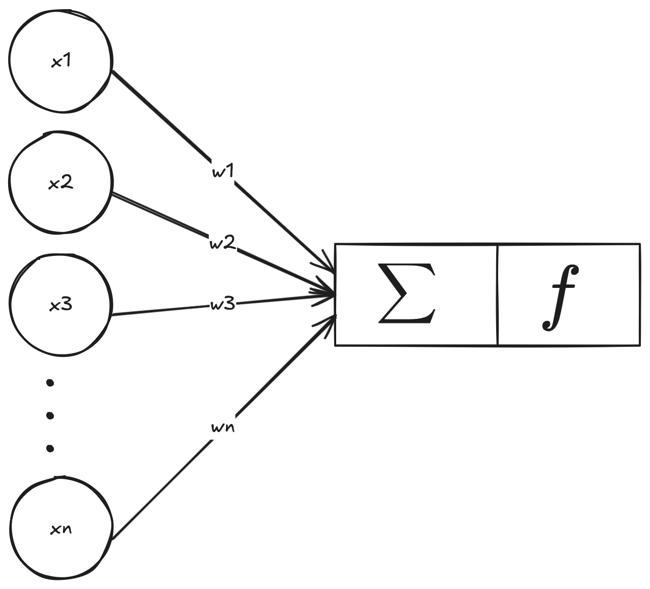
Where x1..xn are the inputs, and w1..wn are the weights.
Inputs and Weights
Every piece of information that enters the neuron ($x$) has an associated weight ($w$):
- A positive weight acts like an excitatory synapse (amplifies the signal).
- A negative weight acts like an inhibitory synapse (reduces or blocks the signal).
The “knowledge” of a neural network isn’t stored in a database — it’s encoded in these weights. So when we say a neural network is “learning,” we mean it’s adjusting these numbers until the output makes sense.
The Sum Function and the Dot Product
The neuron’s first step is to sum everything it received, in a weighted fashion. We multiply each input by its corresponding weight and add up the results:
$$ Sum = (x_1 \cdot w_1) + (x_2 \cdot w_2) + \dots + (x_n \cdot w_n) $$
In programming, doing this loop manually for thousands of inputs would be slow. To solve that, we can use the Dot Product. Instead of iterating, we treat the inputs and weights as two vectors and let linear algebra do the work all at once.
In Python, using the NumPy library, this is done with the .dot() method, which is optimized in C and far faster than any native for loop.
Activation Function
After summing everything, we need to decide whether the neuron fires or not. That’s what the Activation Function is for.
In the classic Perceptron, we use the Step Function. If the sum is greater than a threshold, it returns 1 (fired). Otherwise, it returns 0.
Practice
Let’s see how all of this works in practice:
import numpy as np

# Input features
inputs = np.array([1, 7, 5])

# Neuron weights
weights = np.array([0.8, 0.1, 0.0])

THRESHOLD = 0.1


def weighted_sum(inputs, weights):
    """Calculates the weighted sum of the inputs."""
    return inputs.dot(weights)


def step_activation(value, threshold):
    """Step activation function."""
    return int(value >= threshold)


if __name__ == '__main__':
    weighted_sum_result = weighted_sum(inputs, weights)
    print(f"Sum result: {weighted_sum_result}")

    output = step_activation(weighted_sum_result, THRESHOLD)
    print(f"Did the neuron fire? {output}")
With just a few lines, we’ve replicated the basic behavior of a nerve cell. But then you might ask: how are these weights defined in the first place? How does the algorithm know it should be 0.8 and not 0.2?
That brings us to the concept of Machine Learning — the heart of neural network training.
Types of Learning
Before we can adjust weights, we need to understand how a machine learns. There are three main approaches:
- Unsupervised learning: the algorithm tries to find patterns on its own in unlabeled data (e.g., grouping customers by purchasing behavior).
- Reinforcement learning: based on trial and error. The model receives “rewards” for correct actions and “penalties” for mistakes (e.g., an AI learning to play a game).
- Supervised learning: we provide the input data along with the correct answer. The model’s goal is to learn to map one to the other.
This post focuses on supervised learning.
Example: Fish vs. Whale
Imagine we want to classify fish and whales. Our inputs (features) could be the animal’s size and whether it breathes air.
If we tell the neuron the animal is huge and has lungs, we say: “For these values, the correct answer is 1 (Whale).”
If it calculates 0 (Fish), it knows it was wrong and needs to adjust.
Weight Adjustment
In the context of a neural network, learning is nothing more than minimizing error. This process uses a classic technique called the Perceptron Learning Rule. The cycle follows a simple logic:
- The neuron makes a prediction (with randomly initialized or zeroed weights).
- We calculate the error: $error = correctAnswer - predictedAnswer$.
- We adjust the weights so that, next time, the error is smaller.
The Update Formula
The Perceptron Learning Rule uses the following formula to update each weight:
$$weight_{new} = weight_{current} + (\eta \cdot input \cdot error)$$
Where $\eta$ is the Learning Rate, which controls the “step size” of each adjustment. If it’s too high, learning becomes unstable. If it’s too low, the neuron takes forever to learn. Values like 0.1 or 0.2 are common.
Note: in more robust models, there’s an extra parameter called Bias, which acts as a weight for an input that is always 1, allowing the neuron to shift its decision boundary. To keep things simple, we’ll focus only on the weights here.
Practical Case 1: AND Operator
We can see this in action with the truth table of the logical AND operator. The goal is for the neuron to fire (1) only when both inputs are 1.
| $x_1$ | $x_2$ | Class (Correct) |
|---|---|---|
| 0 | 0 | 0 |
| 0 | 1 | 0 |
| 1 | 0 | 0 |
| 1 | 1 | 1 |
Training
If we start with weights at 0 and a threshold of 1, the neuron will get the last case wrong ($1, 1 \to 1$), since the sum will be $0$.
- Error detected: 1 (correct) - 0 (predicted) = 1
- Adjustment: using a learning rate of 0.1, the weights climb a little each round (or rather, each epoch).
- Convergence: after a few epochs, the weights will reach 0.5. Now, when $x_1=1$ and $x_2=1$, the sum is $0.5+0.5=1.0$. The neuron hits the threshold and finally gets it right!
The interesting part is that we never programmed the AND rule. We just gave it examples, and the neuron “discovered” the weights needed to satisfy the logic.
Implementing the Training Loop
Translating all this theory into a Python script, the key piece is the while loop: it represents the network’s effort to repeat the process (the epochs) until the total error reaches zero — meaning it gets every combination in the AND table right.
import numpy as np

LEARNING_RATE = 0.1
THRESHOLD = 1.0

# AND logic gate truth table.
inputs = np.array([
    [0, 0],
    [0, 1],
    [1, 0],
    [1, 1]
])

outputs = np.array([0, 0, 0, 1])

# Initial perceptron weights.
weights = np.array([0.0, 0.0])

def step_activation(value):
    # Activation function: fires if it reaches the threshold.
    return int(value >= THRESHOLD)

def predict(sample):
    # Dot Product followed by Activation.
    weighted_sum = sample.dot(weights)
    return step_activation(weighted_sum)

def train():
    total_error = 1  # Start with an error to enter the loop

    # Loop until the network gets 100% of samples right (zero error)
    while total_error != 0:
        total_error = 0
        print(f"Epoch start - weights: {weights}")

        for sample, expected_output in zip(inputs, outputs):
            predicted_output = predict(sample)
            error = expected_output - predicted_output

            # Accumulate absolute error to control the loop
            total_error += abs(error)

            # Perceptron learning rule:
            # Update weights proportionally to the error and learning rate
            weights[:] += LEARNING_RATE * sample * error

        print(f"Epoch end - weights: {weights}")
        print(f"Total errors: {total_error}\n")

if __name__ == '__main__':
    train()
    print("Neural network trained")

    # --- Demonstration ---
    print("--- Testing the trained network ---")
    for sample in inputs:
        result = predict(sample)
        print(f"Input: {sample} -> Predicted output: {result}")
Running this code, we can watch the weights “climbing” from $0.0$ to $0.5$. In the final step, the network runs the test and the predicted outputs match the AND truth table exactly — the neuron now “understands” the logical operator.
Practical Case 2: OR Operator
Unlike AND, where both inputs need to be 1, the OR operator only requires one input to be 1 for the neuron to fire.
| x1 | x2 | Class (Correct) |
|---|---|---|
| 0 | 0 | 0 |
| 0 | 1 | 1 |
| 1 | 0 | 1 |
| 1 | 1 | 1 |
The code to train OR is identical to AND — just change the outputs array:
# OR logic gate truth table.
outputs = np.array([0, 1, 1, 1])
With the same settings, the network will converge to weights that satisfy the OR logic.
Practical Case 3: Fish vs. Whale (Generalization)
Unlike the AND operator, which is an exact logical rule, real-world data is messier. To illustrate this, let’s train the Perceptron to tell a Fish from a Whale using two features: Size (0 to 1) and whether it has Lungs (1) or gills (0).
import numpy as np

LEARNING_RATE = 0.1
THRESHOLD = 0.5

# Dataset: [Size, Breathes with Lungs (0=No, 1=Yes)]
# Labels: 0 = Fish, 1 = Whale
inputs = np.array([
    [0.1, 0], # Small fish
    [0.2, 0], # Medium fish
    [0.8, 1], # Large whale
    [0.9, 1]  # Giant whale
])
outputs = np.array([0, 0, 1, 1])
weights = np.array([0.0, 0.0])

def step_activation(value):
    return int(value >= THRESHOLD)

def predict(sample):
    return step_activation(sample.dot(weights))

def train():
    total_error = 1
    while total_error != 0:
        total_error = 0
        for sample, expected in zip(inputs, outputs):
            error = expected - predict(sample)
            total_error += abs(error)
            weights[:] += LEARNING_RATE * sample * error

if __name__ == '__main__':
    train()

    # Testing with a Dolphin (medium size, but has lungs)
    dolphin = np.array([0.5, 1])
    res = predict(dolphin)
    print(f"Dolphin result: {'Whale/Mammal' if res == 1 else 'Fish'}")
The Dolphin Mystery
When we run this script, the Dolphin gets classified as a Fish. A few conclusions we can draw:
- The algorithm is “lazy”: the Perceptron stops training as soon as it finds any line that separates the data. If it decided that “being huge” is the main criterion, it will ignore the lungs for medium-sized animals.
- Lack of diversity: we never gave it examples of medium-sized animals with lungs. To the neuron, whales are just “giant things.”
- Bias: without this parameter (mentioned in the note above), the neural network has less flexibility to shift its decision boundary, which can lead to generalization errors like this one.
To fix these issues, we’d need a richer dataset or a more complex architecture.
Practical Case 4: XOR Operator
Earlier, when we talked about the Origin, I mentioned that the Perceptron triggered an “AI Winter” — and the main culprit was the XOR (Exclusive OR) operator.
Unlike OR, XOR only fires if exactly one of the inputs is 1. If both are 1, the output must be 0.
| x1 | x2 | Class (XOR) |
|---|---|---|
| 0 | 0 | 0 |
| 0 | 1 | 1 |
| 1 | 0 | 1 |
| 1 | 1 | 0 |
Just try swapping the outputs array for this:
# XOR truth table - the Perceptron will fail here!
outputs = np.array([0, 1, 1, 0])
If you try to train the network with these outputs, you’ll see the while loop run forever — the error never reaches zero.
Why Does It Fail?
The Perceptron is a linear classifier. That means it tries to draw a straight line to separate the zeros from the ones.
With AND and OR, you can draw that line. With XOR, the points are distributed in a way that makes it mathematically impossible to separate them with a single straight line.
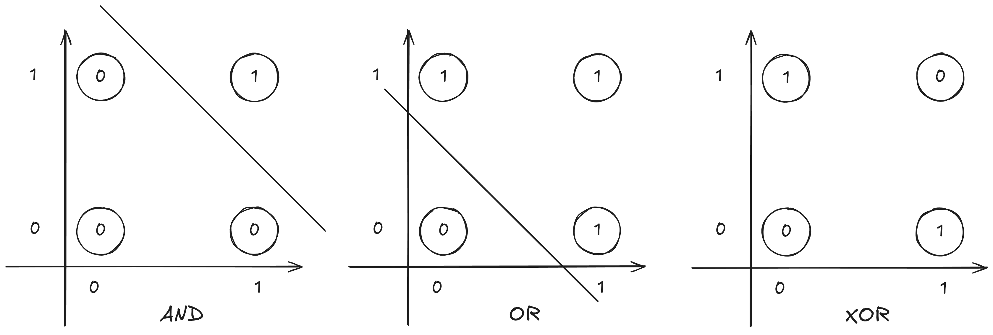
In the XOR case, no straight line can correctly separate the classes.
This was the limitation that stalled the field for years. The solution would only come later, with the addition of hidden layers, giving rise to what we call Multilayer Neural Networks — capable of drawing curves and complex shapes to separate any kind of data.
Conclusion
What Frank Rosenblatt built in 1958 wasn’t just an algorithm, but a bridge. It’s fascinating (and a little unsettling) to think that, nearly 70 years later, these matrix multiplications and weight adjustments are still at the core of the world’s most advanced AI systems.
The Perceptron has its limits: it’s lazy and needs well-prepared data to avoid confusing dolphins with fish. But those limits were the spark that led to Multilayer Neural Networks and Deep Learning. The XOR problem forced the field to stop looking at isolated neurons and start looking at connections.
Modern artificial intelligence is not just a Perceptron at scale. Techniques like hidden layers solve non-linearity, bias adds flexibility, and modern activation functions alongside algorithms like Backpropagation allow learning to flow through deep neural networks. When all is said and done, today’s AI may be frighteningly complex, but the fundamental mechanics that dictate how it learns still began right there, with that first artificial neuron, back in the 1950s.
Thanks for reading, and see you in the next post!